예측 결과 점검
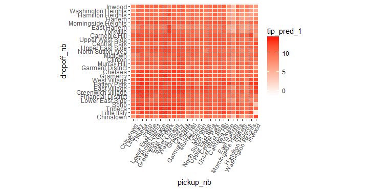
이제 모든 조합에 대한 예측 평균값을 플로팅하여 모델의 예측 결과를 시각화 할 수 있습니다.
ggplot(pred_df_1, aes(x = pickup_nb, y = dropoff_nb)) +
  geom_tile(aes(fill = tip_pred_1), colour = "white") +
  theme(axis.text.x = element_text(angle = 60, hjust = 1)) +
  scale_fill_gradient(low = "white", high = "red") +
  coord_fixed(ratio = .9)
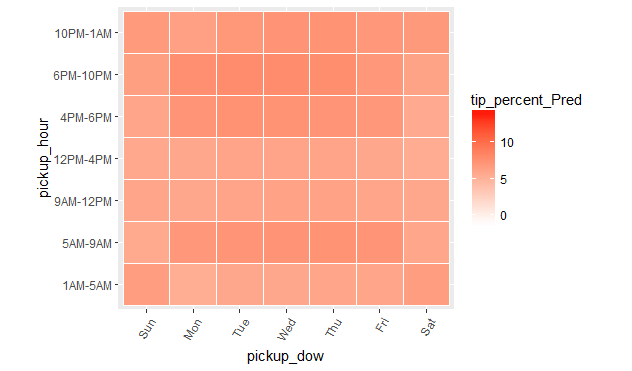
ggplot(pred_df_1, aes(x = pickup_dow, y = pickup_hour)) +
  geom_tile(aes(fill = tip_pred_1), colour = "white") +
  theme(axis.text.x = element_text(angle = 60, hjust = 1)) +
  scale_fill_gradient(low = "white", high = "red") +
  coord_fixed(ratio = .9)